Financial Mathematics Literature Review

Mathematical Finance → Financial Mathematics Literature Review

Random walk and Brownian motion
A random walk is a natural process that can be observed in many fields. Often, random walks have Markov property (that only current position is relevant). And, the observations of many random positions (or random variable) over a period of time lays the foundation of stochastic processes (also called Random processes) because the random variable changes in an uncertain way.

The modern Financial Mathematics has roots in the discovery of the Brownian motion in 1827 by Scottish botanist Robert Brown [1]. The Brownian motion is a stochastic process that models random continuous motion. He observed random motion of microscopic particles resulting from their collision with atoms or molecules in a fluid moving with different velocities and in different directions.

Louis Bachelier 1900 [2], a French Mathematician, was the first who introduced Mathematics of Brownian motion, and compared its trajectories with stock prices behavior and calculated option values. Thus, he developed the theory of option pricing and became pioneer in Financial Mathematics.

Albert Einstein 1905 [3] suggested a mathematical model and expressed that the displacement of a Brownian particle is proportional to the square root of the time elapsed. However, Nobert Wiener 1923 [4] provided the rigorous mathematical construction of standard Brownian motion. Hence, the standard Brownian motion is also called Wiener process.

If we consider a random walk of a variable $z$ , such that $z=0$ at $t=0$ . In the limit $\Delta t \rightarrow 0$ , we say expected change in $z$ when $\Delta t \rightarrow 0$ is 0. And the change in $z$ from time 0 to $T$ is the sum of these very small intervals is also 0. And, according to Albert Einstein the mean displacement (uncertainty in our case) of this type of variable is proportional to $\sqrt{t}$ . So, by the central limit theorem the variable $z$ follows a normal distribution. The resultant process is continuous-time Markov stochastic process called Wiener process (or standard Brownian motion), and can be defined as follows.

Wiener Process
The change in $\Delta z$ during a small period of time $\Delta t$ is

$\Delta z= \varepsilon \sqrt{\Delta t}$

Where $\varepsilon$ has a standardized normal distribution $\varnothing (0,1)$ , and the value of $\Delta z$ for any two different short intervals of time, $\Delta t$ , are independent [5]. The Wiener process we developed has drift rate of 0 and variance rate of 1.

Generalized Wiener Process
In a generalized Wiener process, the drift rate and the variance rate can be set equal to any chosen constants. A generalized Wiener process for a variable $x$ can be defined in terms of $dz$ (considering $dx=adt$ used to indicate $\Delta x=a\Delta t$ when $\Delta t \rightarrow 0$ ) as

$dx=a(x,t)dt+b(x,t)dz$

with expected drift rate of $a$ , and variance rate of $b^2$ .

If we compare the generalized Wiener process with stock process, then it is

$dS=\mu dt+\sigma dz$

where $\mu$ is stock’s expected rate of return, and $\sigma$ is the volatility of the stock price. But, this is not appropriate for stock prices because as we have seen in computing interest

Interest $=Prt$

Where $P$ is current price, $r$ is rate of return and $t$ is time. Here current price is changing in percentage terms.

Geometric Wiener Process
Similarly to the interest formula, for stock prices, we can say, its expected percentage change in a short period of time should be constant (not its expected absolute change). And also, uncertainty about future stock prices is proportional to the current prices. By considering this, we obtain the following stock price process

$dS=\mu Sdt+\sigma Sdz$

This process is known as geometric Wiener process (or geometric Brownian motion).

Ito Process and Ito’s Lemma
Kiyoshi Ito 1951 [6], a Japanese mathematician, derived a very important result to solve stochastic differential equation following Ito process.

Ito process can be defined as, it is generalized Wiener process where parameters are functions of the underlying variable and time, i.e.

$dx=a(x,t)dt+b(x,t)dz$

Using Ito Lemma, we can show that a function $G$ of $x$ and $t$ follows the process

$dG=(\frac{\partial G}{\partial x}a+\frac{\partial G}{\partial t}+\frac{1}{2}\frac{\partial^2 G}{\partial x^2}b^2)dt+\frac{\partial G}{\partial x}bdz$

Option prices depend on stock prices and time. And, if we let $f$ as the price of a call option, then, by using Ito Lemma, we obtain

$df=(\frac{\partial f}{\partial S}\mu S+\frac{\partial f}{\partial t}+\frac{1}{2}\frac{\partial^2 f}{\partial S^2}\sigma ^2 S^2)dt+\frac{\partial f}{\partial S}\sigma Sdz$

Black, Scholes and Merton 1973 [7] created a riskless portfolio of the option and stock to eliminate the Wiener process from the above equation, and obtained Black-Scholes-Merton partial differential equation

$\frac{\partial f}{\partial t}+rS \frac{\partial f}{\partial S}+ \frac{1}{2}\sigma ^2 S^2 \frac{\partial ^2 f}{\partial S^2}=rf$

Final and Boundary conditions
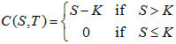
The European call option gives the payoff $S-K$ at $t=T$ when $S>K$ and is worthless otherwise, so the final condition is

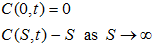
The option is worthless, that is, $C(0,t)=0$ when $S=0$ . And, when the asset price increases without bound, that is, $S \rightarrow \infty$ , the exercise becomes less and less important. Hence, the boundary conditions are

Black-Scholes-Merton Formula
The solution to the Black-Scholes-Merton partial differential equation with these final and boundary conditions is famous Black-Scholes-Merton option pricing formula for European-style call option

$c=S_oN(d_1)-Ke^{-rT}N(d_2)$

Using put-call parity for European option

$c-p=S_o-e^{-rT}K$

We can obtain the formula for European put option

$p=Ke^{-rT}N(-d_2)-S_oN(-d_1)$

Where

$d_1=\frac{ln(S_o/K)+(r+\sigma^2/2)T}{\sigma\sqrt{T}}$

and

$d_2=d_1-\sigma\sqrt{T}$

REFERENCES

Robert Brwon, a brief account of microscopical observations, 1827
Louis Bachelier, Theorie de la Speculation (Gauthier-Villars, Paris, 1900)
Albert Einstein, “Investigations on the theory of the Brownian motion,” (1905)
Nobert Wiener, The average of an analytical functional and the Brownian movement, Proc. Nat. Acad. Sci. USA. 7 (1921), 294-298. And, Differential space. J. Math. and Phys. 2 (1923), 131-174.
Options, Futures and other Derivatives by John C. Hull
Kiyoshi Ito, “On Stochastic Differential Equations”, 1951
F. Black, M. Scholes, “The Pricing of Options and Corporate Liabilities,” (1973)

References

Robert Brown, A. (1827). A brief account of microscopical observations.
Louis Bachelier. (1900). Theorie de la Speculation (Gauthier-Villars, Paris).
Einstein, A. (1905). On the movement of small particles suspended in a stationary liquid demanded by the molecular-kinetic theory of heat). Investigations on the Theory of the Brownian Movement, Dover, New York.
Nobert Wiener. (1921). The average of an analytical functional and the Brownian movement, Proc. Nat. Acad. Sci. USA. 7, 294-298.
Nobert Wiener. (1923). Differential space. J. Math. and Phys. 2, 131-174.
Hull, J. (2015). Options, futures, and other derivatives. Upper Saddle River, NJ: Pearson Education, Inc.
Kiyoshi Ito. (1951). On stochastic differential equations (Vol. 4, pp. 289-302). New York: American Mathematical Society.
Black, F., & Scholes, M. (1973). The pricing of options and corporate liabilities. Journal of political economy, 81(3), 637-654.